Escherly Seeds is the name of a project on which I started working early 2022, intended as a submission to an online generative art platform called Art Blocks. As the name suggests, it’s an ode to one of my favorite artists, M. C. Escher.
Algorithmic art, to me, shares a kinship with the natural sciences – understanding the complexities of a subject often enhances your ability to appreciate it. By explaining the details, I hope you feel the same.
Some parts might be difficult to follow without a bit of graphics programming knowledge, but it does give insight behind certain aesthetic choices.
Penrose’s triangle
This project started out as an attempt to reverse-engineer the famous Penrose triangle illusion which Escher so often used. The shape is an example of an impossible object and depends on the viewer’s perception of depth being ambiguous. In Escherly Seeds this is done by using isometric projection which can be interpreted as viewing an object or geometry in a way where all three axes of space are of equal length.
A Penrose triangle can be decomposed into a collection of 12 cubes, viewed in isometric projection. The golden cubes have faces that are independently placed in depth.
Let’s say you have a glass cube. How do you view it in a way that all 12 edges of the cube are of the same size? If you place it flat on a table and look at it from above, you will have shortened the axis that goes into the table, you cannot see it’s length at all! Now if you twist it by 45 degrees to the left such that it rests on an edge, you will will have gotten closer. All edges now have a length, but they’re still not equal; the edges on the top and bottom will be a little bit shorter. We can remedy this by once again twisting the cube in a way that it’s perfectly resting on its corner. Imagine trying to balance a cube on your finger, and what that would look like from above. That’s isometric projection.
Except not really, because we’ve forgotten a crucial element: depth. The cube’s edges that are further away from your eye will be slightly smaller. Your eyes – fortunately – are limited in this respect. True isometric projection is outside the realm of human perception, because the rays that emanate from the viewing position have to be be parallel. If one had a fictional camera that was infinitely far away, and yet infinitely far zoomed in, you will now see the cube’s sides to be of equal length. More importantly, the cube remains the same size no matter how far it is from the viewer.
In Escherly Seeds a Penrose triangle is composed of isometric cubes with extra functionality. The solution is to allow certain cubes to have disconnected faces, where their distance from the camera will be arranged to make it appear that the triangle is continuous, as seen in Fig. 1. Rotating these faces around their local axes reveals their true locations. Note that this technique only works if the triangle’s sides are of a minimum length of four, but this does mean we can easily create any impossible shape as long as it follows this hexagonal grid.
Generating the tree
It was surprisingly tricky to create a robust method for generating something tree-like. I am a huge fan of the space colonization algorithm when it comes to procedural botany, but that doesn’t work given the constraints of our geometrical environment. My method can be split into two parts.
The generative algorithm is divided into two phases: an initial recursive growth phase and a trunk-carving phase.
I wrote a function which “grows” a branch, and called it recursively#. The branch has a starting location, and is also constrained by the width and height set at the beginning of the algorithm. What gives it variety is that the probability weights for which direction and magnitude the branch will grow in is decided pseudo-randomly. For example, if there is a higher probability of the branch growing sideways as opposed to upwards, the tree generally looks fatter and bushier as is the case in Fig. 2. Once the first branch, or stem, is finished, each node itself will call the same branching function with a different probability distribution#.
You might think that’s probably good enough for a surrealist tree. It’s decent, I guess. The method still had a habit of looking too blocky and boring, and I noticed this especially when I was experimenting with aesthetically pleasing techniques for partitioning the tree’s crown. The tree just would not interpolate nicely, it didn’t flow.
In the second part a trunk is carved out from this initial structure# following a ruleset tuned to make the trunk weave as much as possible. A path would be traced out starting from the root until a node was reached that was connected to more than two others. From there two possibilities could happen:
- If the node was a simple fork, the shortest path would be deleted from the structure#.
- If the node was of a higher degree, this junction would be split# such that the trunk could continue growing. In Fig. 2 this scenario is shown in red.
This would continue until certain conditions were met#, eventually halting the growth of the trunk. There were way more subtleties to this than I had anticipated, particularly the strict ruleset required to split the junctions in an appropriate way#. Certain combinations of angles look strange, and these angles influence whether the trunk should go under or above the junction, all the while trying to maximize the weaving aesthetic of the trunk. But a benefit of this convoluted method is that the tree will often have an impression of flowing back down into itself, which I thought was very pleasing.
From pencil to 3D
I wanted Escherly Seeds to have a good narrative, and one way I thought this could be done effectively is if the tree begins as a paper sketch and then grows into its 3D form. It took months to figure out the best way to do this. Earlier prototypes had a “hole” in the paper from which the cubes emerged, but I wanted the legit blend from 2D to 3D just like Escher’s Drawing Hands. (I initially thought this would count as an extra optical illusion, but apparently this effect does not qualify.)
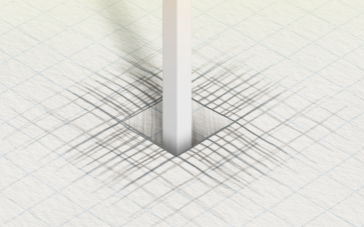
Earlier prototypes had a faux-hole from which the tree would emerge.
The trick was to render the roots in a separate “sketchify” pipeline and then manually blend it with the tree inside a composition shader. Fading from one to the other within the same viewport required a lot of fine-tuning. The sudden rotation at the transition was crucial too because it hides unpleasant discontinuities.
There is a simple technique which can create a pencil-like effect, although it only works for outlines. You calculate the slope of the luminosity at every point in your texture: the sharper the edge, the darker the stroke of your pencil. For a human touch, distort your coordinate system with some noise. A few of these layers with different amplitudes and frequencies, and you’ve got a decently looking effect at moderate computational cost.
But in order to be able to properly transition from pencil to 3D, I needed more granular control of the pencil strokes. Since luminosity is a scalar value I could just store different components into their own RGBA channel and process them separately.
- R. The luminosity of the top faces of the cubes are stored here.
- G. This channel contains the side faces of the cubes. Toggling this on makes the paper appear to have depth.
- B. The short trunk of the tree gets its own channel, because those strokes needed to be faded on top to make the illusion work.
Once we have these layers separated and sketchified acccordingly, we can compose our Escherly metamorphosis in the composition shader, which I show here step-by-step.
An incremental reconstruction of how the composition shader mixes each layer, smoothly blending the roots with the tree.
- We calculate a paper texture in real-time by using two noise texture lookups and calculating its gradient. I added parallel sketchpad lines to sell the effect a little better#.
- We use the the alpha channel of the tree along with the root’s stem (which we stored in the blue channel) to mask these paper lines#.
- The pencil strokes of the top faces are blended into the paper first#.
- Then the fill colors of the entire root system are also blended in#.
- The shadow effect is, just like the rest of the structure, completely non-sensical. A Penrose triangle has ambiguous depth so casted shadows are paradoxical. But, somehow, it works but just doing a Gaussian blur of the alpha channel, rotating it a bit, and adding a subtle perspective#. The same mask as in step 2 is used to make the shadow appear to be behind the trunk.
- The background fog is just a random color gradient which the paper and shadows are radially blended into#.
- Now we superpose the 3D tree layer#, making sure to smoothly interpolate the transition along the length of the trunk.
- Finally, we polish off the transition by overlaying the pencil strokes of the stem and side faces#.
Optimizing it for mobile
Mobile GPUs are often limited by fill-rate, so full-frame effects tend to be avoided by mobile WebGL programmers. I found this out the hard way. Escherly Seeds was prototyped on a mediocre laptop and I was surprised to find that the framerate dropped drastically once I ported it to my phone. The bottleneck was coming from the various pixel shaders responsible for the metamorphosis effect. Functions which I had assumed to be rather rudimentary could sometimes add milliseconds per frame!
So I had to really reduce and optimize my shaders, which, inevitably went at the cost of some visual quality. But in return you gain the ability to interact smoothly via touch. Of course, I tried to prerender as much data as possible. But the crucial insight was that by splitting the rendering pipeline into different stages#, I could distribute the computational load over the duration of the animation.
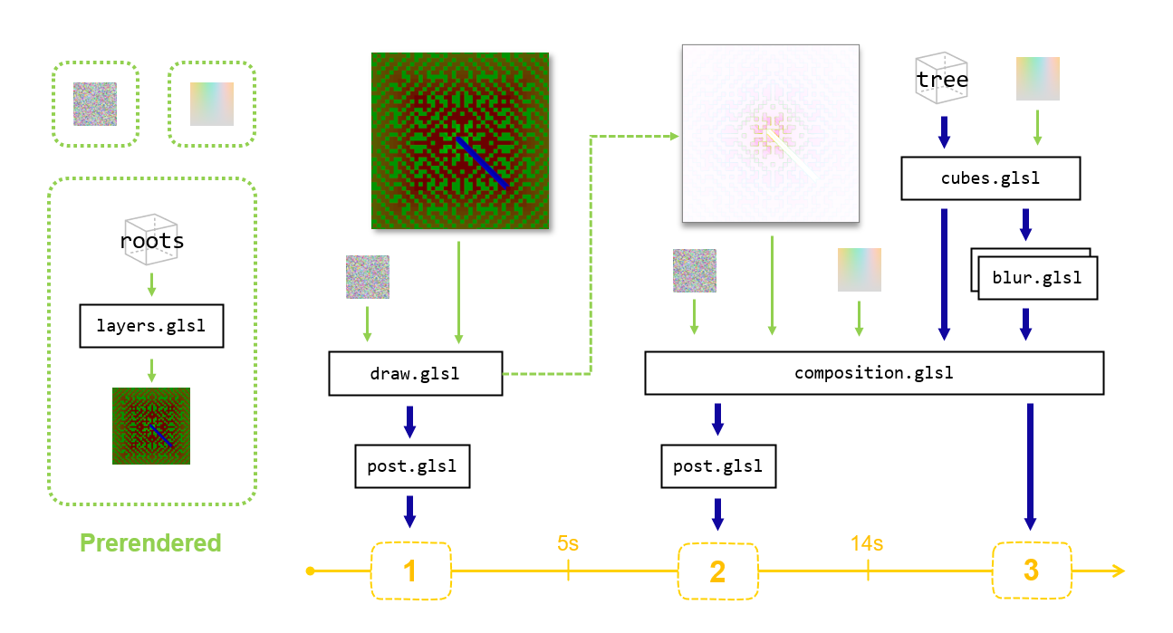
This is an overview of the shader pipelines used during the execution of Escherly Seeds. Several textures are prerendered to speed up runtime, shown on the left of the figure. The roots are also prerendered into a large MSAA-enabled texture. Static data are represented by light green arrows and dynamic data streams are shown by dark blue arrows. The yellow axis denotes the flow of time, from which you can see that the pipeline has three stages which switch at 5s and 14s, although the only difference between the last two is the bypassing of the post.glsl shader. blur.glsl is shown with a stacked rectangle because the blurring is separated into a vertical and horizontal stage. The dashed green arrow emerging from draw.glsl points to another texture which is technically also prerendered, but since it stores animation data at the transition between pipelines it was more logical to place it in that location.
Two small 64x64 texture are first pre-generated on the CPU. The first is a typical 4D noise texture#, just like those found on ShaderToy. The second texture is a color lookup table# which uses Inigo Quilez’s color palette technique to define a hue in the X axis. The Y-axis determines the saturation. The lookup texture is used both for the cubes’ color and the background fog. These two textures are shown in the top left corner of Fig. 5. Also, a larger FBO is used to prerender the RGB-separated layers of the root’s cubes#, as explained in the previous section.
The first section of the animation takes place mostly in draw.glsl# where a paper texture is viewed from the top while the pencil strokes are slowly faded in. Each pencil stroke needs 8 texture lookups#, bringing the total to 24. Some extra basic processing is done too, like radially fading the strokes out. Another benefit of separating this part of the animation is that this means that no expensive coordinate transformations are included in the sketch effect calculations. At 5s, right before the rotational transition, draw.glsl emits another FBO where each RGBA channel has pre-sketchified layers#, including fill colors. (Technically, this part is also prerendered#.)
The second section is calculated mostly within composition.glsl#, rotating the sketchified texture and blending several layers as shown in Fig. 4. Importantly, all the expensive pencil effect texture lookups have been off-loaded, otherwise this fragment shader would not run in real-time on mobile GPUs.
The last step of the pipeline is post.glsl# and only runs from 0 to 14s. The naming is a bit of a misnomer because color-grading and tone-mapping# are already done invididually inside draw.glsl and composition.glsl. A more appropriate name would be intro or fadein because all it does is enable the subtle transition from greyscale to full-color#, or the occasional chromatic explosion# effect. Once the intro is finished, it just serves as pointless overhead and is bypassed#.
Modular cubes
Each face of each cube is given a set of parameters which can be modulated in real-time, determining certain visual aspects. On the GPU the data have the following layout#:
                // .xxxxxxxx.yyyyyyyy.zzzzzzzz.wwwwwwww.
in vec4 pos;    // |        translation       | faceID |
in vec4 shape;  // |           scale          |  fold  |
in vec4 turn;   // |      rotation axis       |  angle |
in vec4 cpar;   // |   hue  | chroma | roughn |  alpha |
in vec4 tpar;   // | invert | texpar |.................|
You can see the first three vectors as representing a specialized transformation matrix, with translation, rotation, and scaling applied to each face#. Not all values in these vectors are used for this purpose, however. An integer faceID is stored in the value pos.w to allow a small trick needed to not overcomplicate the instanced rendering technique. This integer corresponds to one of the cube’s six faces and will rotate and flip the quad accordingly#. I decided to leave the translation and rotation axis static because the ruleset for their variety would have been too complicated: you would need a system to avoid overlapping primitives, for example.
There is also an extra function to the value stored in shape.w. Each face has the ability to be folded in such a way that it adopts the shape of another polyhedron. To allow for this modularity, I wrote a function# which subdivides the face’s quad congruently to the necessary creases. Depending on the polyhedron – several of which can be seen in Escher’s print Stars – the vertex shader will be compiled# with a function which does the appropriate folding.
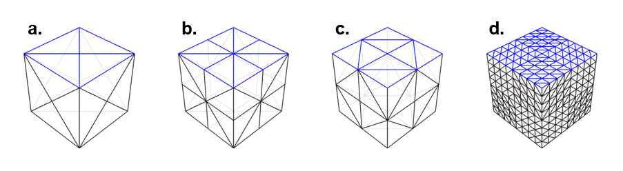
These 4 tesselations can be folded into 7 different polyhedra; a. Rhombic dodecahedron, ‘Star’; b. Stella octangula, Escher’s solid; c. Compound of cube and octahedron; d. Octahedron, Sphere.
The colors of the cube’s faces are derived from the values in cpar. The first two (cpar.xy) are used as input coordinates to a texture lookup table defining a color. I used the PBR model to light the faces of the cube, except I modified the equations to only allow for fully metallic surfaces#, meaning that only roughness is necessary: stored in cpar.z. The remaining value controls the face’s opacity.
The last 4-vector tpar only uses the first two values; these parameters are used to give the artwork some special features.
More optical illusions!
Escherly Seeds has a maximum of three optical illusions.
Somewhat accidentally I discovered that there’s a rather simple way to implement another optical illusion! Once all the cubes’ faces are projected isometrically inside the vertex shader, you can toggle its Z coordinate# causing an inversion through the viewing plane. It’s as if the cube flips in perspective, making it seem like you’re looking at it from behind. Escher also used this illusion prolifically, most notably in his lithograph Hol en Bol.
(Fun fact: The pithy title is originally in Dutch and translates directly to “Concave and Convex”. For some reason, however, the widely accepted title seems to have these words in reversed order.)
The first parameter in tpar toggles this effect by taking the values +1 or -1. For this to work seemlessly with instanced rendering, however, it must be accompanied by a reordering of the faces#. The light direction vector is also adjusted to make sure that the shadow is still somewhat logical at the base#. Another restriction is that this inversion causes a discontinuity between paths: either the whole tree is inverted, or just an isolated segment.
The last parameter tpar.y is used to modulate a visual pattern shown on the faces inside of the fragment shader. A few procedural textures are possible#, but a specific one enables another optical illusion similar to what’s called the Spinning dancer. This function will discolor the faces and make them translucent in a randomly generated periodic pattern#.
Here comes the dirty trick: if you rotate the cube with depth-testing disabled you’ll have faces which overlap in a very confusing manner, making it difficult to determine the direction of rotation. The downside of this, however, is that visibly correct rotation is not possible anymore so all other rotations inside the tree are disabled#. But it adds another layer of surrealism to the artwork.
Synchronization physics
One of the benefits of using real-time techniques is that it places another fun toolbox at your disposal: physics simulations. Here is where my background came in handy, and I experimented with various models. I settled on the Kuramoto model which is probably most known for being able to simulate the synchronization of fireflies, but there are other examples too. You know when an audience applauds and then, slowly, the claps take on a rhythm? Same thing.
A popular science educator Veritasium made a video about it, and he interviews Steven Strogatz who is a well-known academic in this field. The equation takes on the following form:

The symbol θi is the phase of oscillator i which has a natural frequency given by ωi. Each cube has a randomly distributed frequency and an internal phase which controls its visual parameters. The second term determines the coupling, which, in this case, only extends to its next-door neighbors. So the summation Ni can go from 1 to 6 depending on the connectedness of the cube. K is the coupling constant and it determines how strongly the cube’s phases are attracted to each other.
The cubes usually synchronize only partially as restricted by their topology, forming waves which look like breathing. Highly connected locations will synchronize more quickly. To make it interactive, I added an extra term where the coupling constant is dependent on the distance x from the cube to your pointer:

Kp is just a smooth function which is very large at proximity and decays to zero with distance. And it attracts the oscillator to a constant value of π which is usually where the animation is at its most interesting. Your finger becomes a brush with which you can force regions into synchrony. This does make undoing the synchronization rather difficult but you’ll find that some regions, like long loops, give you some room to play.
I spent a lot of time testing more complex models, but in the end simplicity won. I tried amplitude oscillators (a generalization which couples both phase and amplitude) which looked really cool, but a few edge cases caused an effect called amplitude death. Too risky. Neuron models like Hodgkin-Huxley just appeared twitchy and nervous. Chaos sounded like a fun idea, but, in practice, it tended to look messy.
By the way, anyone curious about using complex dynamical systems creatively should check out the wonderful website complexity-explorables.org. Just keep in mind that interesting physics doesn’t always mean “pretty” physics.
Trees with individuality
Escherly Seeds starts out as a simple sketch and then grows into a surrealist 3D tree, full of color and movement. It was a metaphor for how artistic mediums evolve over time – Escher planted something that continues to grow to this very day. That narrative was very dear to me, but it depended on a rigid composition, making it a challenge to maximize the diversity of the series. My strategy was to partition the crown# of the tree into visually distinct regions with a selection of dynamic styles.
Again, it surprised me how many limitations there were; it was a real balance between maximizing variety and playing whack-a-mole with the occasional outlier. Smooth transitions between regions were particularly fussy.
Botanical regions
It made sense that the elements furthest away from the root would be special; the endpoint(s) should represent the conclusion of the transformation. I calculate a distance matrix# using the Floyd-Warshall method, allowing me to quickly find the shortest path between nodes, and thus the furthest away nodes.
- When it was possible to create a tight loop starting from the last node, and provided it didn’t break any other rules#, that region is called fruit#. It made sense for another reason: sometimes loops could cut off other nodes from connecting to the trunk#, resulting in an unpleasant discontinuity. This happened rarely, but I saw a poetic opportunity: the fruit had ripened with its own seeds!
- If the furthest away nodes were placed in corners, for a maximum of two, we could segment those into flowers#. If one of these was hidden behind a trunk I would just flip it# back front.
- A fail-safe way to segment the tree is to just combine the last few bins of a distance histogram into one and create a region of foliage called leaves#. This could always be combined with either of the first two botanical features. (Fruit and flowers are mutually exclusive.)
Once these regions are determined, they are visually separated by limiting the size of its neighboring nodes. Additionally, a color gradient is interpolated along the distance from these regions# with variable setpoints and slope. The type of functions for color mattered a lot, exponential curves looked significantly better than smoothstep, for example.
Feature examples
Here is a collage of several of these botanical features and styles, zoomed in so you can see the details more clearly.
- A flower with the Mobius# style, inspired by Escher’s use of hyperbolic geometry. A Möbius transformation with randomized parameters is compiled into the composition shader# and can be light or dark. Pay attention to another lighting trick: lines on the tree are offset from those in the background. We also see the more common sticks# style of the branches.
- A highly connected patch of leaves which will strongly synchronize their folding into Escher’s solid. In this style called metal# the rotation axes are parallel and both the folding and specularity will modulate simultaneously to get a discoball effect. (Some polyhedra show this effect more strongly than others.)
- We see a style that fruit can adopt called morph# where the XYZ scaling is smoothly interpolated over the cycle without any rotation. Here you can most clearly see that colors are always darkened with a decrease in size#. Note that the fruit is inverted compared to the branches; an extra optical illusion.
- Occasionally the algorithm will be able to find two flowers in the structure, which is quite rare. The polyhedron here is called star and if you look closely you’ll see the added effect of a radial gradient shader.
- Flowers can have a glass# style containing an extra kinetic optical illusion. The texture’s coordinates are translated during rotation to give a kaleidoscope effect with an ambiguous rotation direction. Note that the opacity is also accurately projected in its shadow.
- These leaves have the zoom# style which tries to mimic a camera’s defocus effect. There’s an inverted trunk optical illusion here too.
- Leaves with stella octangula as the selected polyhedron. The rotation axes are randomized and the specular reflections are muted giving a matte# style.
- This output is quite rare because it contains seeds! These are always black and spherical, only modulating in size#. The animation style of the fruit is called twist# where the rotation axis is congruent with the cycle, and turns a full period. The specularity and opacity both slightly modulate during rotation. Fruit with seeds will also always have a cyclical hue#.
- Another style of fruit is called flat# which has grey sticks in one direction, while the rest of the loop rotates half a period in a perpendicular direction with increased specularity. This fruit is also inverted! The branch style is also called flat# but does only a reduction in size and rotates a full period. The leaves use a shader to create the toon# style.